2. Getting Started
Example data can be found into the datasets/gettingstarted/ folder: coord.cor, observ.obs.
2.1. Input Files
All coordinates and observations files are text files with fields delimited by any number of spaces or tabs. Blank lines are overlooked.
Example:
* Station 1
7 S1  S3    0.0000  0.0020  0.001   *no heights
5 S1  S2  391.3030  0.0020  0.001  0.0000 0.0000
6 S1  S3   99.9280  0.0020  0.00   1.6170 1.5630
6 S1  S2   99.8060  0.0020  0.00   1.6170 1.5790
@monday.obs
2.1.2. Subfiles
Subfiles can be included in .cor or .obs files with a @ character preceeding their filename path relative to the current file.
2.1.3. File Paths
Comp3D data files can be located in any directory with the following restrictions:
spaces are not allowed in relative subfiles paths since they will be interpreted as field separators
Windows, unlike other operating systems, is case-insensitive, so wrong case can be used for subfile inclusions, but this will not work on other OS
2.2. Create a Project
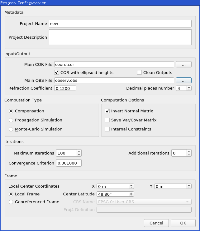
With the .cor and .obs files, you can create a new project. In the graphical user interface, select Project>New, choose a file name (to make things simple in the same folder as the data files) and fill in the Project Configuration form as described in Project Configuration. The mandatory parameters are the root .cor and .obs files and the input frame (for the getting started example, the default local frame is sufficient).
The new project is then automatically loaded into the main window.
2.3. Main Window
Once the project is loaded in the graphical user interface with Project>Open, the project reading messages are shown.
Use Configuration button to make changes on project parameters, Reload to reload input files, Start Compensation/Propagation/Monte-Carlo to start the action or View Log to open the html report file.
The graphical user interface contains two main tables (as described in Main Tables):
list of points
list of observations
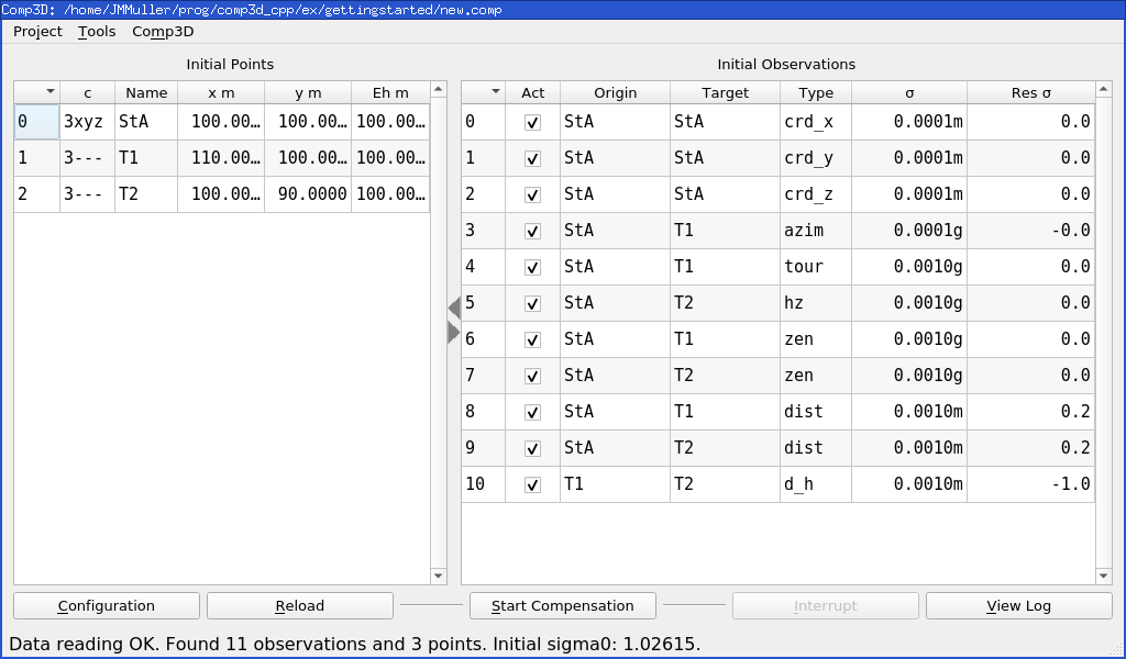
Observations can be activated or deactivated using the Act field (see Changing Observation Status).
2.4. Html Report
The html report is automatically generated at the end of computation. It can be loaded in the system default web browser with the View Log button. Using this button before computation, as expected, it will open the report in the initial state before computation.
The computation report shows the map, the initial and final coordinates and the list of observations with many statistical indicators.
For more details and explanations, see Computation Report.
2.5. Quick Review of an Example
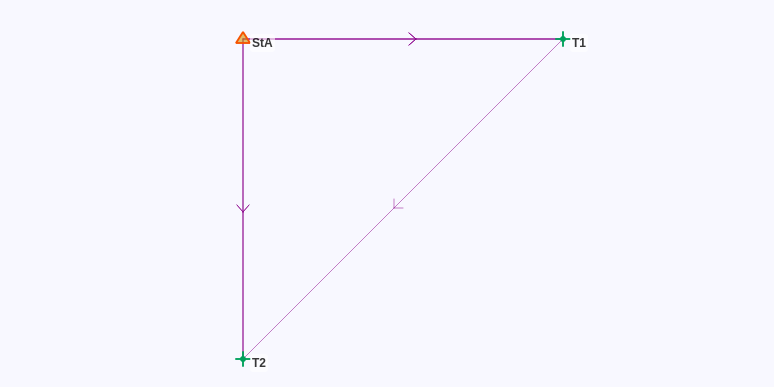
The example in datasets/gettingstarted/ folder is simply one total station (StA) measuring two targets (T1 and T2). A height difference between T1 and T2 is added to give some redondancy.
2.5.1. Example of .COR File
See example .cor file in datasets/gettingstarted/coord.cor
1 StA 100 100 100 0.0001 0.0001 0.0001 * known point
In this example, only one point is declared, it provides minimal information to set the position of the project.
The point StA was chosen as all the other points can easily be determined from it in this project. The other two points will be inferred from the .obs file.
For more details and explanations, see COR File.
2.5.2. Example of .OBS File
See example .obs file in datasets/gettingstarted/observ.obs
8 StA T1 100 0.0001   * azimuth to fix orientation of figure

* topometric observations
7 StA T1   0 0.001  * horizontal reference
5 StA T2 100 0.001  * horizontal angle

6 StA T1  100 0.001  * vertical angle
6 StA T2  100 0.001

3 StA T1  10 0.001  * distance
3 StA T2  10 0.001

* leveling between targets
4 T1 T2 0.001 0.001
In this example, an azimuth between two points is used to give the orientation of the whole figure. Then we have total stations observations from StA to T1 and T2, and a leveling measurement between T1 and T2 to give some redondancy.
Note
In Comp3D, all linear observations values are in meters and angular observations values are in grads (gons).
For more details and explanations, see OBS File.
2.5.3. Computation
When the project is loaded, the coordinates of the undeclared points are initialized, if possible. Then, the initial residual of every observation and the initial \(\sigma_0\) is given.
The final \(\sigma_0\) is obtained after computation. In this example, it is close to 1, meaning that the weights of the observations are coherent with their residuals.
For more details and explanations, see Computation.
2.1.1. Comments
The
*character defines a comment that goes up to the end of the line.The comments associated to an observation or a point will appear as such in the .html report file.